An Introduction to Training Algorithms
for Neuromorphic Computing and On-line learning
On-line Learning
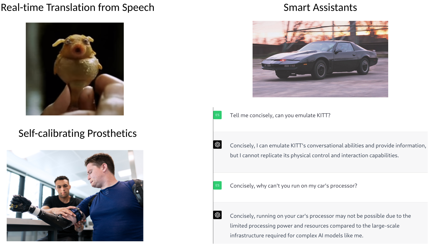
Technologies to solve above exist learning important, but running them at the edge remains a challenge
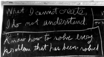
The Physics of Computation

|
The constraints on our analog silicon systems are similar to those on neural systems: wire is limited, power is precious, robustness and reliability are essential.
Mead, 1989
|

|
|
The constraints on our analog silicon systems are similar to those on neural systems: wire is limited, power is precious, robustness and reliability are essential.
Mead, 1989
The Brain exploits Physics, Why is that useful?
Computer and Brain Engineering Stack
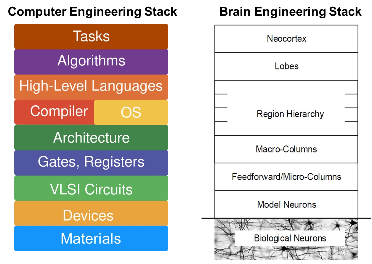
The equivalent computer engineering principles in biological brain are not known
J.E. Smith, “Reverse-Engineering the Brain: A Computer Architecture Grand Challenge” ISCA Tutorial 2018
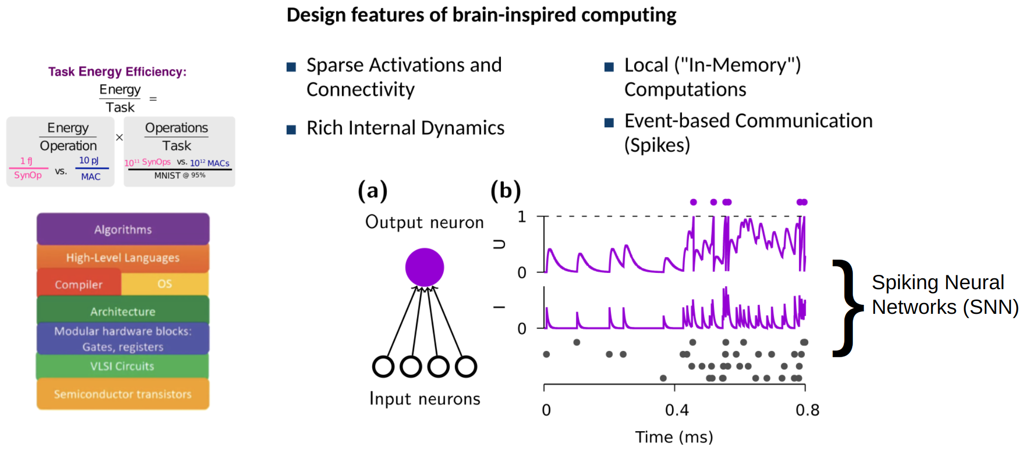
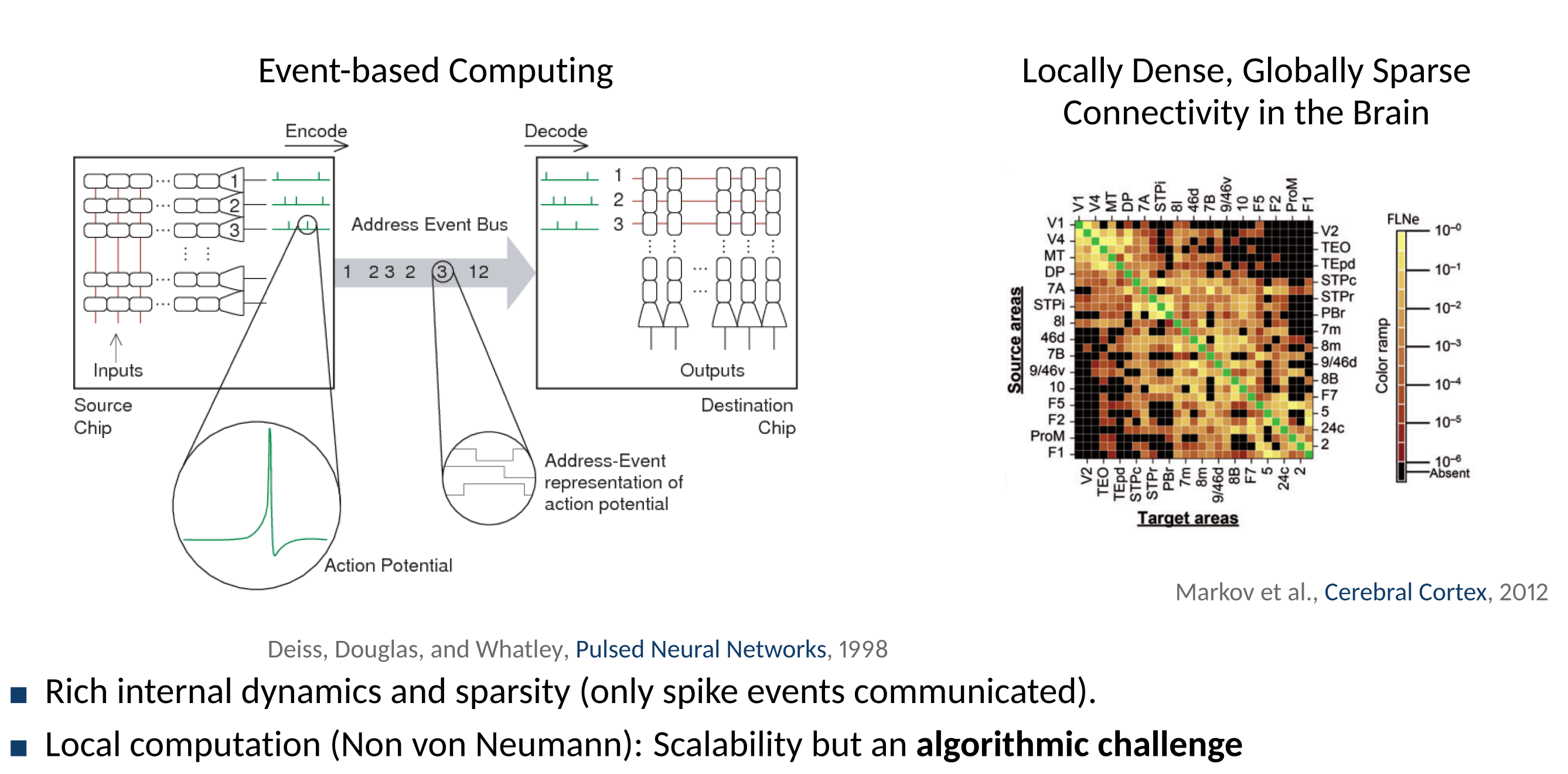
Design Features of Brain-Inspired Computing
Brain Anatomy Constrains Neural Computation
Douglas and Martin 2012
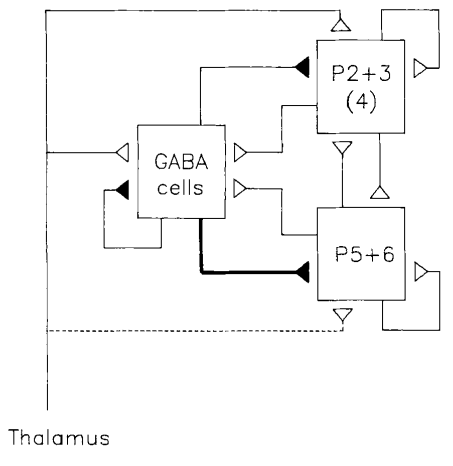
Local circuits have strongly excitatory and inhibitory interactions
$\rightarrow$ canonical microcircuit, EI balance, Attractor networks
Douglas et al. 1989
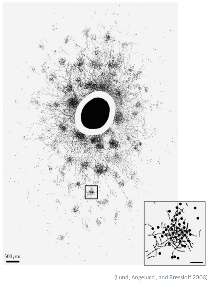
Local and Recurrent connectivity: Pyramidal cells project to distant (few mm) clusters of target cellsInterconnected canonical microcircuits could be universal approximators, but no theory yet to build a functional cortical sheet
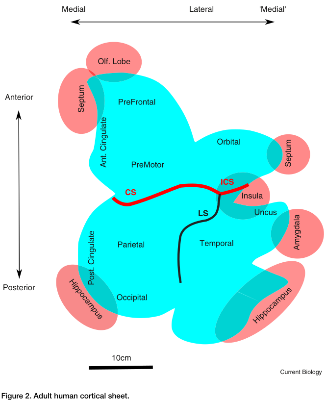
Cortical Connectivity
- White-matter connections between cortical areas
- Highly inhomogeneous and area specific
- Hierarchical organization with layer-specific feedforward (bottom-up) and feedback (top-down) connections

Budd and Kisvarday 2012
Allen Brain Map
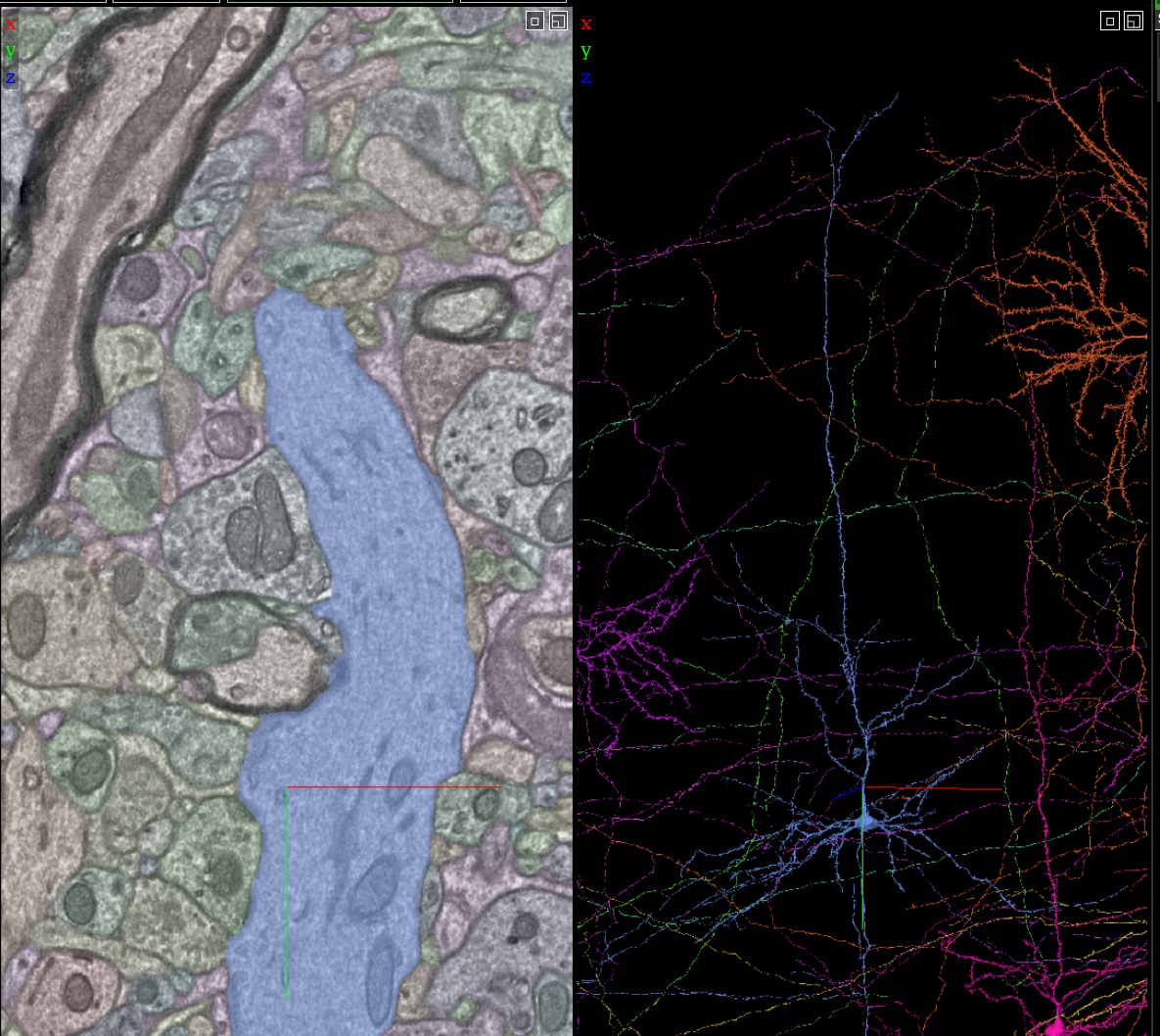
Massive efforts to map the brain at different scales

Credit: https://www.microns-explorer.org/phase1
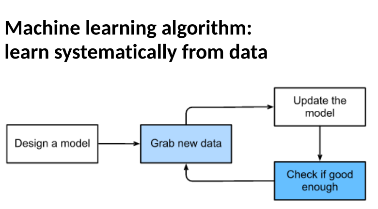
Neuromorphic Computing as a Technology
Machine Learning
This tutorial:
1. Recurrent Neural Networks Basics and Spiking Neurons
2. Can machine learning rules be used as a learning model in biological neural networks and brain-inspired hardware?
3. Brains learn continually, but deep networks are trained from scratch. Can we do better?

Neftci et al. 2019
Neural Networks
We can connect Perceptrons together to form a multi-layered network.

-
If a neuron produces an input, it is called an input neuron
If a neuron's output is used as a prediction, we will call it an output neuron
If a neuron is neither and input or an output neuron, it is a hidden neuron
- Increased level of abstraction from layer to layer
The Gradient Back-Propagation Algorithm
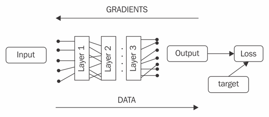
- Forward-propagate to compute $y^{(k)}$ for all layers $k$
- Compute loss and error
- Back-propagate error through network, i.e compute all $\mathbf{\delta}^{(k)}$
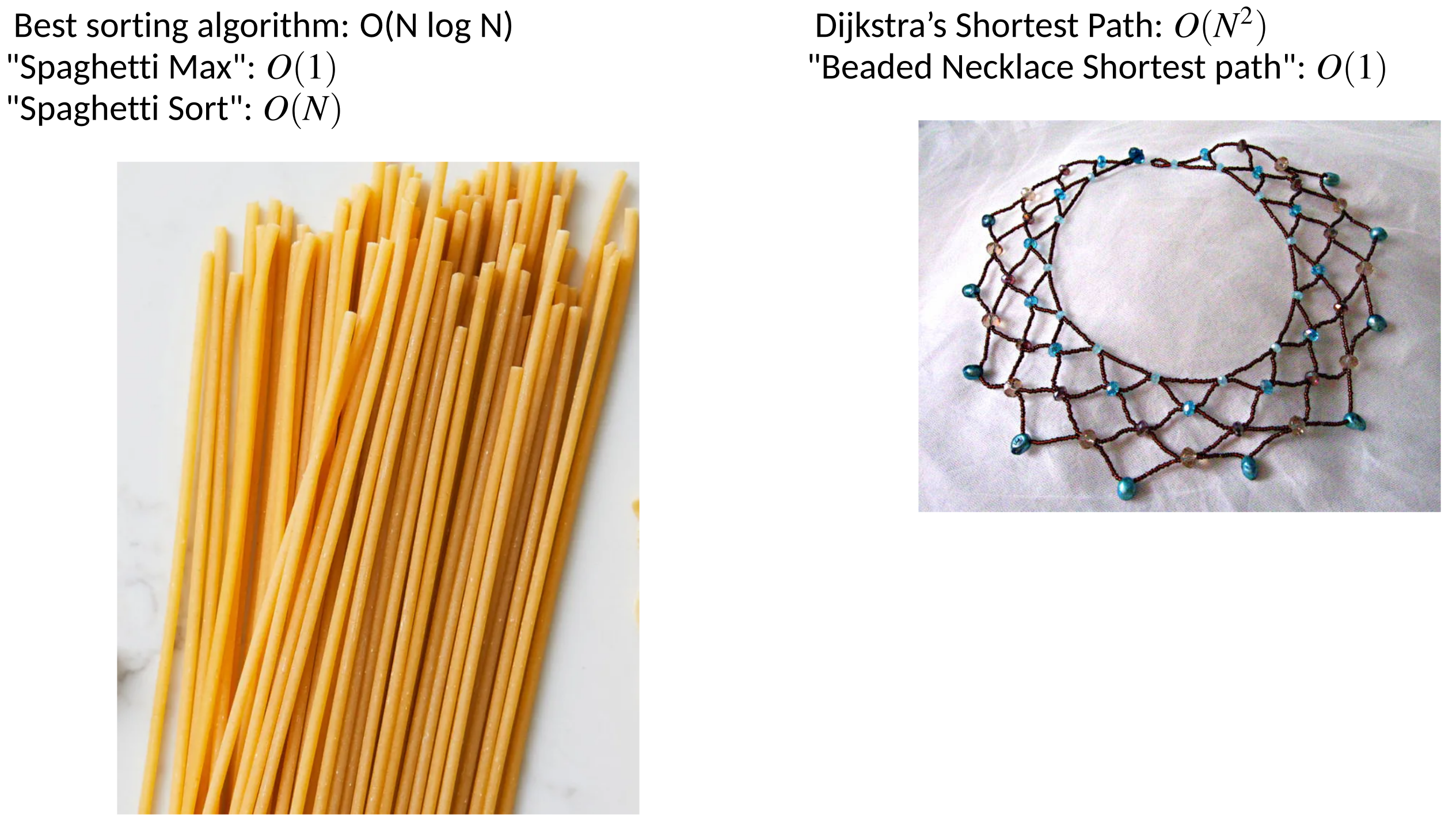
Where Brain-Inspired Computing Beats Conventional Computing
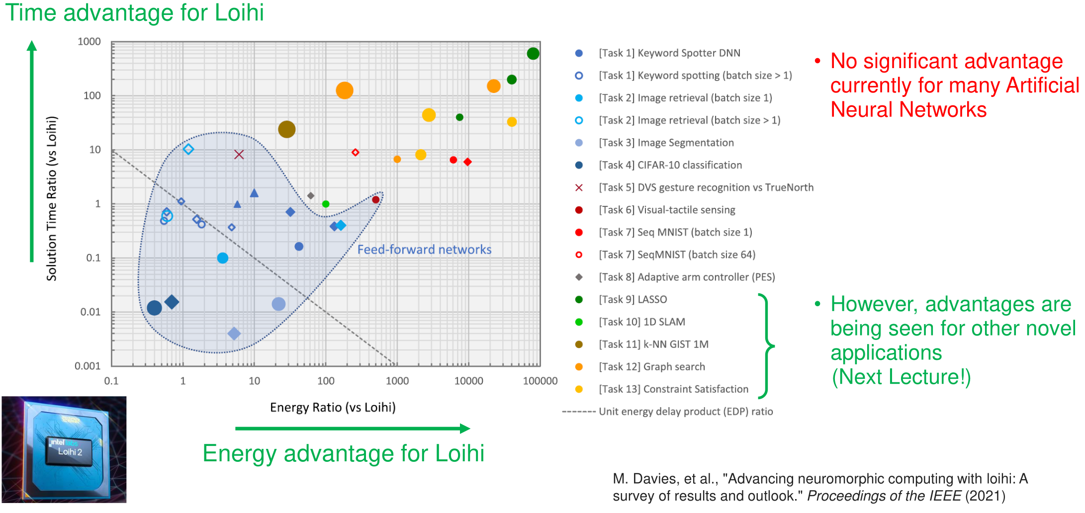
Tasks 7-13 features time-dependent data and recurrent connections
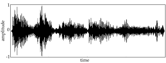
Time-Dependent Data
-
Almost all real-world data is sequential (embedded in a time-like dimension):
- Videos

- Audio
- Text

How to Deal with Variable-Sized Dimensions?
Time is a variable dimension. Feed-forward neural networks static dimensions. There are two ways to deal with this:
-
Fix the size, truncate (pad) the data that has a larger (smaller) dimension. For example for size 2:
- EOS is a special symbol meaning end-of-sequence.
- Recurrent neural networks are designed to deal with such data. They include recurrent (feedback) connections
[[1, 5, 6], [3,4], [3]] -- [[1, 5], [3,4], [3, None]] -
Once the size is fixed, a feed-forward neural network can be used
[[1, 5, 6], [3,4], [3]] := [[1,3,3],[5,4, EOS],[3,EOS, None] Recurrent Neural Networks (RNNs) in Neuroscience
- Short-term memory implemented using recurrent connections
- The majority of connections in the brain are recurrent

Douglas and Martin, 1989
... physically mapped the synapses on the dendritic trees (...) in layer 4 of the cat primary visual cortex and found that only 5% of the excitatory synapses arose from the lateral geniculate nucleus (LGN)
Binzegger et al. 2004
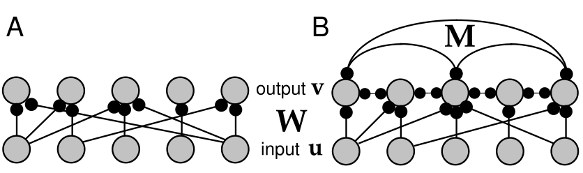
Recurrent Neural Network in Deep Learning
- Recurrent Neural Networks introduce recurrent connections
- What is the consequence of having recurrent connections in the neural network graph for training?
- Errors (gradients) must be propagated through the loop!
- If the variable size dimension is time, errors need to be propagated to the past.
https://colah.github.io/posts/2015-08-Understanding-LSTMs/
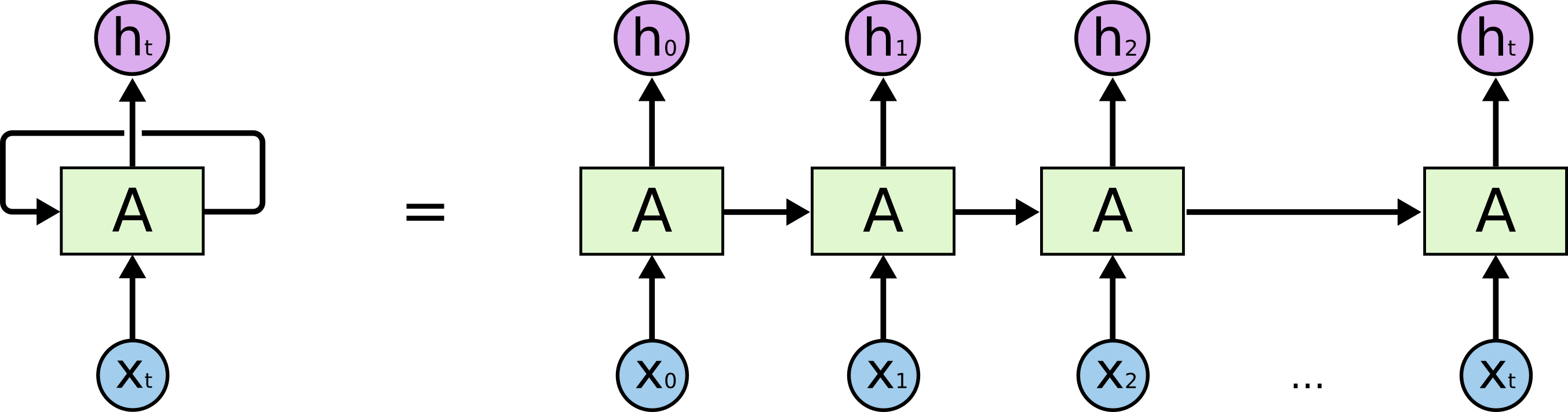
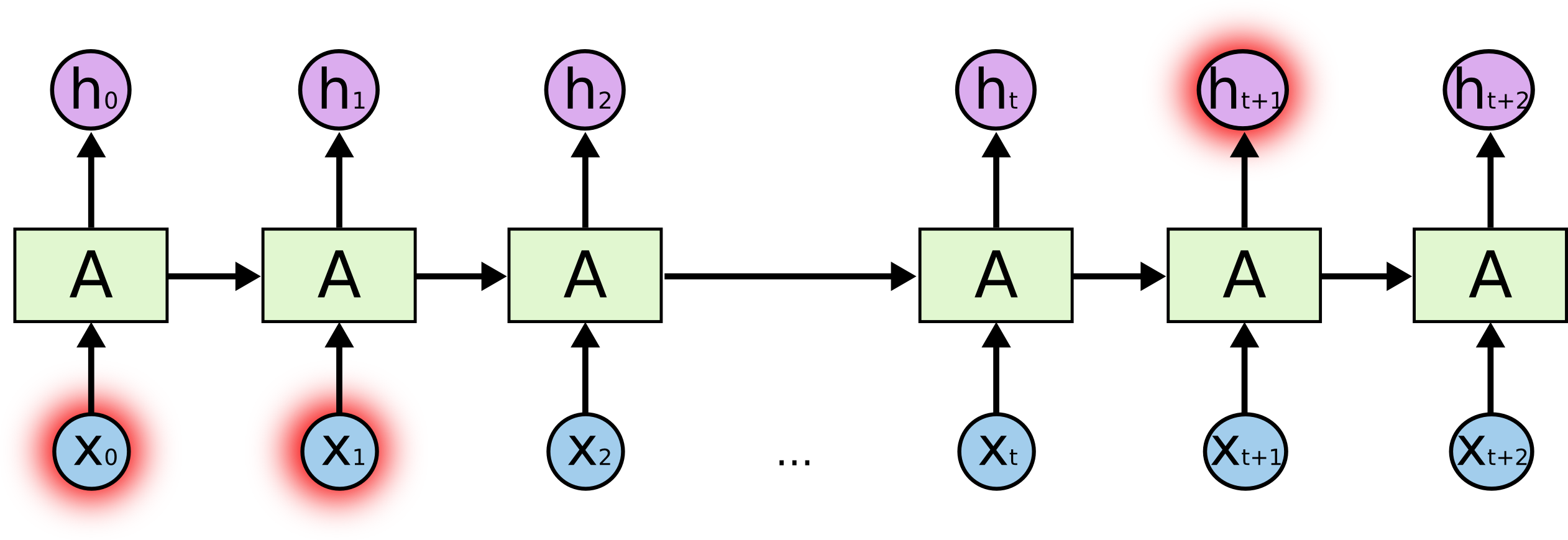
Recurrent Neural Networks in Deep Learning
-
RNNs can be unfolded to form a deep neural network
The depth along the unfolded dimension is equal to the number of time steps.
An output can be produced at some or every time steps.
Example Tasks
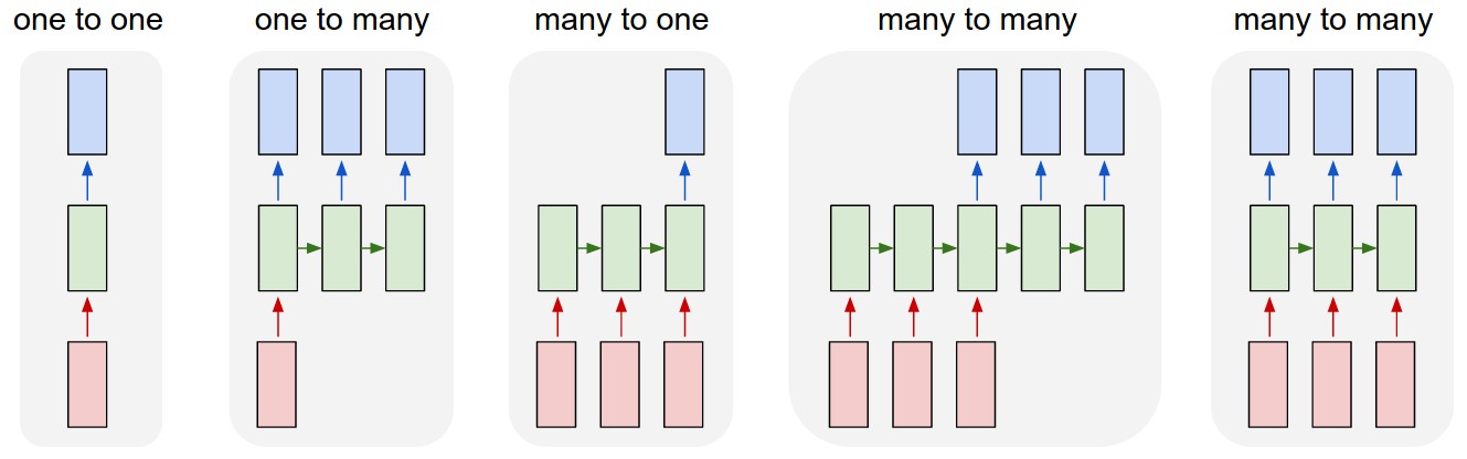
Examples: Depending on the output structure, different problems can be solved:
- Many-to-one: Classification, Sentiment analysis
- Many-to-many: Machine translation
- One-to-many: Image captioning
- One-to-one: Time series prediction
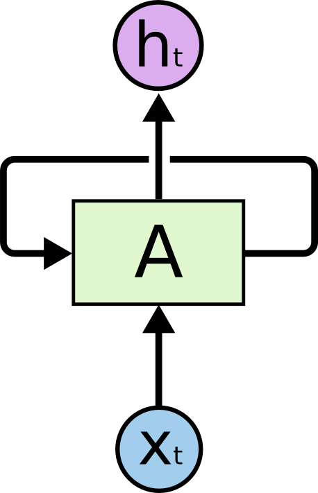
Simple Recurrent Neural Network
- Also called Elman RNN, these are the simplest RNNs.
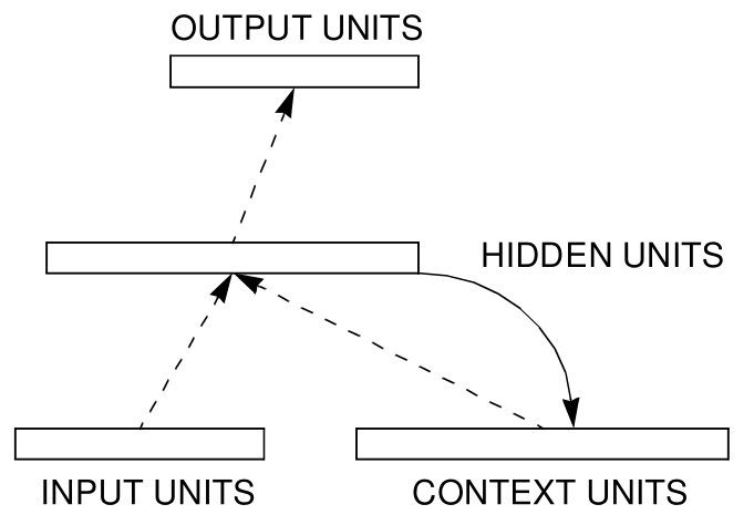
Elman, Finding Structure in Time, 1990
$$ \begin{split} h_t = \text{tanh}(W_{ih}\mathbf{x}_t + W_{hh} \mathbf{h}_{(t-1)} ) \end{split} $$
- A simple recurrent network is simply a network whose output feeds back to itself
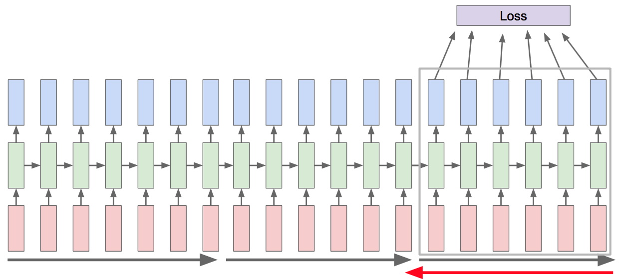
Unrolled Neural Network
- We can use the same training framework as feed-forward networks by unrolling the variable-size dimension.
- We apply back-propagation to the unrolled network. This is called Back-Propagation-Through-Time (BPTT).
- Conceptual difference wrt feedforward networks: Parameters are shared along the horizontal axis.
https://colah.github.io/posts/2015-08-Understanding-LSTMs/
Challenges in Computing Gradients in RNNs
-
We can use the same training framework as feed-forward networks by unrolling the variable-size dimension.
https://colah.github.io/posts/2015-08-Understanding-LSTMs/
There are two problems when computing gradients-
Memory grows with sequence length
Vanishing (or exploding) gradients: in simple RNNs, memory decays exponentially, so it cannot learn long-term dependencies in practice.
Solving the Memory problem: Truncated Backpropagation
- Truncated BPTT: Backpropagate $h$ steps in the past
Complexity of Gradient-Based Algorithms in RNNs
- $n$ number of neurons
- $L$ number of time steps
- $h$ representing the number of prior time steps saved (truncation)
- BPTT space complexity is $O(nL)$
- Real-time Recurrent Learning (RTRL) is an online alternative to backpropagation (more on this later)

Williams and Zipser, 1995
RNNs and the Vanishing Gradients Problem
-
We can use the same training framework as feed-forward networks by unrolling the variable-size dimension.
https://colah.github.io/posts/2015-08-Understanding-LSTMs/
There are two problems when computing gradients-
Memory grows without bounds
Vanishing gradients
The Vanishing Gradients Problem
The temporal separation between targets and inputs makes training difficult. This is called the temporal credit assignment problem
- Short-term dependencies

- Long-term dependencies
https://colah.github.io/posts/2015-08-Understanding-LSTMs/
- Vanishing gradients: in simple RNNs, memory decays exponentially, so it cannot learn long-term dependencies in practice.
Bengio et al. 1994
Perfect Integrator
- We can construct dynamics that keeps a perfect trace: $$ h_t = h_{t-1} +f(x_t) $$ but then we would be overwhelmed by noise and spurious inputs
- The central problem for training networks with memory: choose which information to remember.
He was, let us not forget, almost incapable of ideas of a general, Platonic sort. Not only was it difficult for him to comprehend that the generic symbol dog embraces so many unlike individuals of diverse size and form; it bothered him that the dog at three fourteen (seen from the side) should have the same name as the dog at three fifteen (seen from the front). His own face in the mirror, his own hands, surprised him every time he saw them (...) He was the solitary and lucid spectator of a multiform, instantaneous and almost intolerably precise world.
Funes the Memorius, Jorge Lui Borges
But how can we know what to remember?
Forget Gates
- Forget gates make storing and forgetting dynamic:
$$
x_t = \sigma(a_t) \odot x_{t-1} + f(a_t)
$$
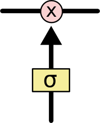

- If $\sigma(a_t)=1$ we remember perfectly, at $\sigma(a_t)=0$ we erase memory
- $\sigma(a_t)$ is a layer of neurons that determines we remember.
- Forget gates are the basic building blocks of all "modern" RNNs
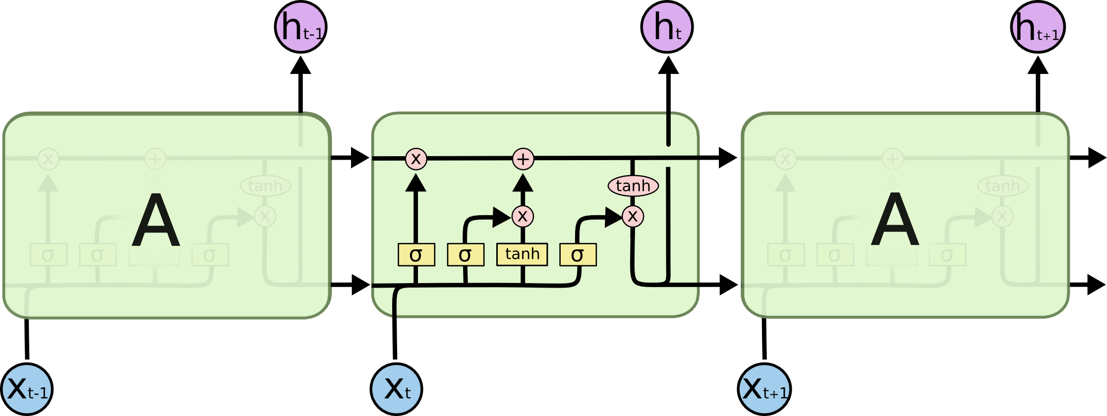
Long-Short Term Memory
-
The LSTM builds on the idea of conveying the hidden state without modification.
The LSTM is the solution to the long term dependency problem proposed by Hochreiter and Schmidhuber in 1997. It is still widely used today.
- ResNets are essentially feedforward versions of LSTM networks
Long-Short Term Memory
https://colah.github.io/posts/2015-08-Understanding-LSTMs/
- The top horizontal line is the memory state, $C_t$
Long-Short Term Memory Equations
-
The choices in LSTM are arbitrary, several variants of LSTMs exist
LSTM models (and variants) are built in machine learning frameworks (e.g. PyTorch)
Memory with optimal polynomial projections
- Is it possible to keep a history of $f(t)\in\mathbb{R}$ at every time step $t$ using leaky integrators?
- Yes: function approximation using coefficients of orthogonal basis functions.

- Project (compress) a representation of this history into space spanned by orthonormal polynomials. Minimization of the following : $$ || f-g ||_\mu := ( \int_{0}^{t} f(s) g(s) \mathrm{d}\mu(s) )^{\frac12}, \quad g(t) = \sum_n c_n(t) g_n(t) $$
- ... leads to dynamics $\frac{\mathrm{d}}{\mathrm{d}t}\mathbf{c}(t)$
(HiPPO, Gu et al. 2020), (Voelker et al. 2019)
State Space Models
- HiPPO is similar to a state-space model (SSM) of a linear system, used in control theory and signal processing
- Maps a $1-D$ time series to a $N-D$ latent space $$ \begin{align} \frac{\mathrm{d}}{\mathrm{d}t} \mathbf{x}(t) &= {A}(t) \mathbf{x}_t + {B}(t) {u}_t \\ {y} &= {C}(t) \mathbf{x}_t + {D}(t) {u}_t \end{align} $$
- With $N$ polynomials, the system requires $O(N^2)$ time for each step
- SSM input is a scalar: for vector inputs, need to use several independent SSMs in parallel, even slower!
- If matrices ${A}, {B}, {C}, {D}$ are time-invariant, the system is called linear time-invariant (LTI)
- In this case, equivalent to a convolutional system: can be implemented efficiently and parallelized on GPUs $$ \begin{align} K(t) &= C \exp(t A) B\\ y(t) &= (K \ast u) (t) \end{align} $$
Structured State Space Models (S4)
- HiPPO/SSM does not scale well. Structured State Space Models (S4) solves this problem via :
- Structure: Diagonalize the matrix $A$ via an approximation (Diagonal Plus Low-Rank). Diagonal means computation is $O(N)$. $A \in \mathbb{C}$
- Linear Time Invariance: $A, B, C, D$ are time-invariant Representing the SSM as a convolution
- Training: optimize the parameters $A, B, C, D$
- One S4 per input channel, resulting the following neural network structure:

(Gu, Goel, Ré, 2021; Smith et al. 2023)
Structured State Space Models (S4)
- Improvement compared to structure used in HiPPO
- Outperforms several other models on long range prediction tasks
| Pathfinder (feed pixels sequentially) |
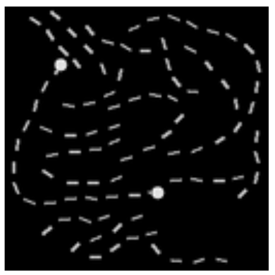
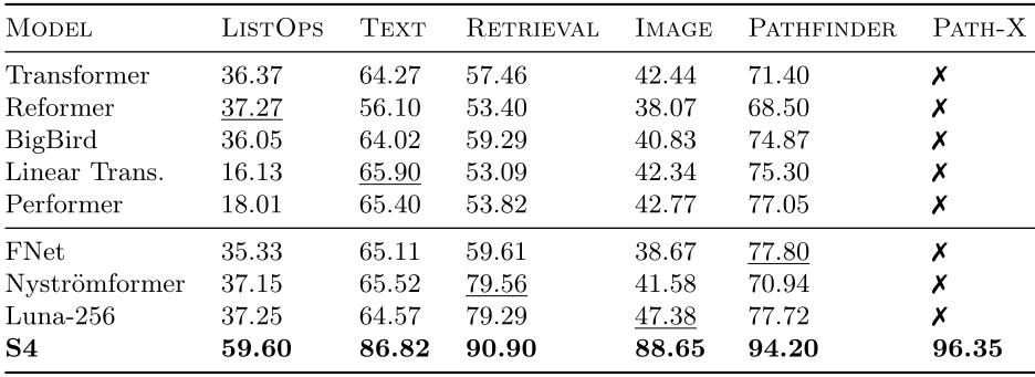
(Gu, Goel, Ré, 2021)
Bringing Back Gating with "Mamba"
- But S4 lost the ability to dynamically adapt (gate) inputs and memory. This was a crucial feature in the LSTM
- Mamba is a recent model that combines the best of both worlds: the ability to adapt memory and the efficiency of S4, at the cost of the convolutional representation
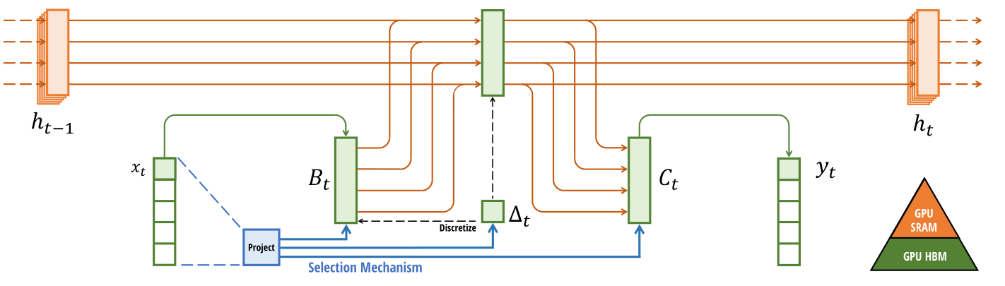
- Strong emphasis on hardware suitability by utilizing the memory hierarchy, fused operations and parallel scan
- Mamba is competitive with transformers on LLM tasks and beyond
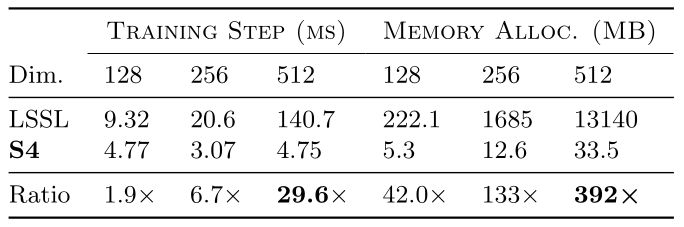
Hardware Utilization in RNNs on TPUs
RNNs are computationally expensive and slow to train due to
- Vanishing gradients problem
- Sequential nature of the computation
- Memory storage: need to store intermediate states
- Memory bandwidth: limited data reuse
- As a result, low utilization of hardware resources
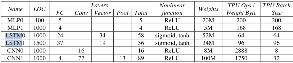
Jouppi et al. 2017