An Introduction to Training Algorithms
for Neuromorphic Computing and On-line learning

PDF Print Layout

Hardware Utilization in RNNs on TPUs

RNNs are computationally expensive and slow to train due to

Vanishing gradients problem
Sequential nature of the computation
Memory storage: need to store intermediate states
Memory bandwidth: limited data reuse
As a result, low utilization of hardware resources
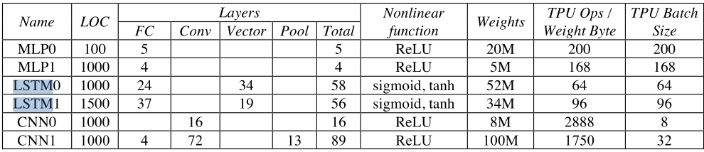
Jouppi et al. 2017

ML/AI Algorithms are Designed fro Existing Software and Hardware

There is a wide gap between AI and Machine Learning

How did the brain inspire AI so far?

Connectionism and learning (e.g. Deep neural networks)
Neural networks inspired by the visual cortex (e.g. ConvNets)
Learning by optimizing a reward (e.g. Reinforcement learning)
Selective Attention (e.g. Self-attnetion)
Recurrent Networks and working memory (e.g. LSTMs)
Episodic Memory (e.g. Memory-Augmented Neural Networks)
Synaptic plasticity and consolidation (e.g. Continual learning)
Transfer Learning ( e.g. Foundation Models)

Many aspects of the brain remain unexplored for computation and AI.

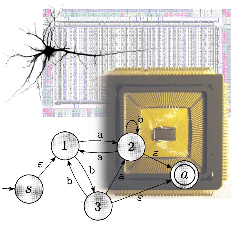
Alternative to von Neumann Computing Architectures

There is no clear separation between memory and processing in neurons.

Credit: Naveeen Verma

Neuromorphic Computing as a Technology

Neuron Models

Neurons are complex dynamical systems. Fully detailed models can be very difficult to simulate and analyze
For simplicity, computational neuroscientists often approximate neuron dynamics with one or more point compartments

This tutorial will mostly focus on the point neuron model, but techniques are applicable to multi-state/multicompartment neurons

Point Neuron Models

A Neuron can be modeled by an equivalent electrical circuit consisting of voltage gates conductances, capacitances and potentials:

Write Eq. 5.7 in Dayan Abbott, but add stochastic term

Dayan and Abbott, 2001

\[ \begin{split} I &= C \frac{\mathrm{d}}{\mathrm{d}t}u + I_{1} + I_{2} + I_L + I_e + I_s \\ I &= C \frac{\mathrm{d}}{\mathrm{d}t}u + g_1(t) (V- E1) + g_2(t) (V- E_2) + g_L (V- E_L) + g_s(t) (V-E_{s}) + I_e \end{split} \]

Hodgkin & Huxley Neuron Model

The Hodgkin-Huxley model is the first biophysically detailed model of the action potential generation
Describes the action potential generation of giant squid axon

A.L. Hodgkin and A.F. Huxley, 1952

Neuron models can be constructed in a similar way by “plugging in” the corresponding currents. $\rightarrow$ "Hodgkin-Huxley type model"

Izhikevich, 2007

Credit: Tom Tetzlaff

Leaky Integrate & Fire (LIF) Neuron

The LIF neuron captures the integration dynamics of a neuron and a minimal model of the action potential generation mechanism.

Integrate-and-fire Neuron Dynamics \[ \begin{split} C \frac{\mathrm{d}}{\mathrm{d}t}u &= - g_L u + I_{syn} + \underbrace{I_{ext}}_\text{e.g. "external input"} \\ \text{if $u>\theta$}&: \text{ elicit spike,} \text{ and } u \leftarrow u_r\text{ during $\tau_{arp}$}\\ \end{split} \]
Action potential (spike) when $u$ reaches $\theta$, reset to $u_{r}$ and clamped during an absolute refractory period $\tau_{arp}$.
Note: Subthreshold dynamics are linear: \[ u(t) = u_{r} + \left((I_{syn} + I_{ext})\ast \kappa\right)(t) \]

Dayan and Abbott book, Section 5.4 and 5.8

Diesmann 2002

Adaptive Leaky & Fire Neurons

Adaptive Leaky Integrate-and-Fire (ALIF) neurons are multistate extensions of the LIF model that can capture a wider range of neural behavoirs:

$$ \begin{split} \tau_{m}\,\frac{{\text{d}}u}{{\text{d}}t} &= f(u)-R\,\sum_{k}w_{k}+R\,I_{ext}(t)\\ \tau_{k}\,\frac{{\text{d}}w_{k}}{{\text{d}}t} &= a_{k}\,(u-u_{\rm r})-w_{k}+{b_{k}\tau_{k}}s(t). \end{split} $$

Gerstner et al. 2014

Synapses

Neurons predominantly communicate with each other through (chemical) synapses.
Synapses can be excitatory or inhibitory.
A neurons typically makes excitatory or inhibitatory connections to other neurons, rarely both (Dale's Law).

Leaky I&F Neuron with Synapse Dynamics

\[ \begin{split} C \frac{\mathrm{d}}{\mathrm{d}t}u &= - g_L u + I_{syn} + I_{ext} \\ \text{if $u>\theta$}&: \text{ elicit spike,} \text{ and } u \leftarrow u_r\text{ during $\tau_{arp}$}\\ \end{split} \] \[ \begin{split} \tau_{s} \frac{\mathrm{d}}{\mathrm{d}t}I_{syn} &= - I_{syn} \\ \text{on presynaptic spike}&: I_{syn} \leftarrow I_{syn}+w \end{split} \]

Action Potential - Basic Unit of Communication

Communication between neurons is primarly mediated by action potentials (’spikes’)
Stereotyped spike shapes (roughly constant in time, across cells, stimulus conditions, species,etc.)
Information is encoded in spike times

Bringuier et al., 1998

Bannister and Thomson, 2007

Credit: Tom Tetzlaff

Firing Rates and Rate-Coding

Rate coding assumes that neurons encode information in their firing rate. Several methods exist to estimate the rate of the neuron:

Mean Firing rate or Spike-Count \[ \frac{1}{T}\int _{0 }^{T }\mathrm{d}t\, s_{pre}(t)= N/T = r \]
Discrete-time firing rate obtained by binning time and counting spikes (B)
Using a window function $h(t)$ (C,D,E) \[ \int _{0 }^{T } \mathrm{d}t\, h(t) s_{pre} = r(t) \]
Note that rate codes are robust to variations in spike times
Rate codes are often used as further simplifications of neurons and populations of neurons

Firing Rate of a Leaky Integrate & Fire Neuron

Firing rate neurons are the building blocks of artificial neural networks

Reliability in Spike Timing in the Brain

Mainen and Sejnowski, 1995

(Left) DC input (no noise) (Right) DC input + white noise

Spiking Neuron in Mixed-Signal CMOS

Credit: Giacomo Indiveri 2024

Spiking Neuron Dynamics

Credit: Giacomo Indiveri 2024

Plasticity and Learning

Spike-Timing Dependent Plasticity

STDP is a synaptic plasticity rule that modifies the strength of a synapse based on the relative timing of pre- and post-synaptic spikes, similarly to the Hebb Rule

Bi and Poo 1998

Jesper Sjostrom and Wulfram Gerstner (2010), Scholarpedia, 5(2):1362.

$W$: Learning Window
$t_i^n$: $n$th spike time of post- neuron $i$
$t_j^f$: $f$th spike time of pre- neuron $i$

$$ \Delta w_j = \sum_{f=1}^N \sum_{n=1}^N W(t_i^n - t_j^f) $$

STDP Visualized

$$ \begin{split} \tau_+{\mathrm{d} \over \mathrm{d}t}P_j &= -P_j + S^{pre}_j\\\\ \tau_-{\mathrm{d}\over \mathrm{d}t} P_i &= -P_i + S^{post}_i\\\\ {\mathrm{d} \over \mathrm{d}t}w_{ij} &= a_+ P_j(t) S^{post}_i + a_- P_i(t) S^{pre}_j \end{split} $$

<h2>Beyond the Hebb/STDP Rule</h2>
  Generalized Hebb Rule: Introduce dependence on pre-synaptic and post-synaptic activities, and the weight itself:

$$
\begin{split}
  \frac{\mathrm{d}}{\mathrm{d} t} w_{ij}(t) &= F(w_{ij}, \nu_i, \nu_j)\\\\
  \frac{\mathrm{d}}{\mathrm{d} t} w_{ij}(t) &= a_0(w_{ij}) + a_1^{pre}(w_{ij})\nu_j +  a_1^{post}(w_{ij})\nu_i + a_2(w_{ij})\nu_i \nu_j + \dots \\\\
\end{split}
$$

<center>
  <table>
  <tr>
    <td>Pre ($\nu_j$)</td> 
    <td>1</td> 
    <td>0</td>
    <td>1</td>
    <td>0</td>
  </tr>
  <tr>
    <td>Post ($\nu_i$) </td>
    <td>1</td> 
    <td>1</td> 
    <td>0</td> 
    <td>0</td>
  </tr>
  <tr class=fragment >
    <td>$\frac{\mathrm{d}}{\mathrm{d} t} w_{ij}(t) \propto \nu_i \nu_j$</td><td>+   </td><td> 0 </td><td> 0 </td><td> 0 </td><td> Hebb's rule </td>

</tr>
  <tr class=fragment >
    <td>$\frac{\mathrm{d}}{\mathrm{d} t} w_{ij}(t) \propto \nu_i \nu_j - c$</td><td>+   </td><td> - </td><td> - </td><td> - </td><td> Hebb's rule with decay</td>
  </tr>
  <tr class=fragment >
    <td> $\frac{\mathrm{d}}{\mathrm{d} t} w_{ij}(t) \propto (\nu_i - c)  \nu_j$ </td><td>+ </td><td> 0 </td><td> - </td><td> 0 </td> <td> BCM (like) rule </td>
  </tr>
  <tr class=fragment >
    <td> $\frac{\mathrm{d}}{\mathrm{d} t} w_{ij}(t) \propto (\nu_j - w_{ij})  \nu_i$ </td><td>+ </td><td> - </td><td> 0 </td><td> 0 </td> <td> SOM rule </td>
  </tr>
  
  <tr class=fragment >
    <td>$\frac{\mathrm{d}}{\mathrm{d} t} w_{ij}(t) \propto \left(\nu_{j}-w_{ij}\nu_{i}\right)\nu_i$</td><td>$\pm$   </td><td> - </td><td> 0 </td><td> 0 </td> <td> Oja's rule </td>
  </tr>
  </table>
  </center>
  <p class=ref>Gerstner and Kistler, 2002</p>

STDP lacks credit assignment

STDP updates only depend on pre-synaptic and post-synaptic activity: No direct influence by task performance
Solution: Add a modulatory signal that depends on task performance
$\rightarrow$ Modulated Hebb Rule

The Concept of Locality

The brain is a physical system constrained by the physical representation of information
For computation to occur on a physical substrate, information much be spatially and temporally local.

Neftci et al. 2019

Locality is relative: global variables can be made available locally if these variables are actively transported to the neuron
Example: STDP is local, but modulated STDP is only local if the $m(t)$ factor is explicitely conveyed to the neuron

Considerations about STDP

Rate-based models are consistent with STDP
Spike-time dependence depends on synapse location wrt soma
The exponential fit of STDP is for computational convenience
Update in original model is relative
STDP is not derived from computational requirements

STDP is a measurement, not an accurate mechanistic model!

Deriving Synaptic Plasticity Rules Using Gradient Descent

\[ \frac{\partial \mathcal{L}}{\partial w_{j}} = \frac{\partial \mathcal{L}}{\partial s} \frac{\partial \mathcal{s}}{\partial u} \frac{\partial \mathcal{u}}{\partial w_{j}} \]

Subthreshold dynamics of a LIF neuron is \[ u(t) = u_{r} + \left(I_{syn}\ast \kappa\right)(t) \]
The $I_{syn}$ can also be similarly written: \[ \begin{split} I_{syn} &= w_{j} \cdot (s_j \ast \kappa_{s} )(t) \end{split} \]

Together we get: \[ u(t) = u_{r} + w_j \left(s_j \ast \epsilon\right)(t), \quad \epsilon = \kappa \ast \kappa_{s} \]
The gradient becomes: \[ \frac{\partial u}{\partial w_j} = \left(s_j \ast \epsilon\right)(t) \]

Note that our derivation relied on the linearity of the subthreshold dynamics: not exact for multiple layers or non-linear neuron/synapse dynamics

Three-Factor Rules

With the surrogate gradient, our learning rule is now: \[ \frac{\partial \mathcal{L}}{\partial w_{ij}} = \frac{\partial \mathcal{L}}{\partial s_{i}} \sigma'(u_i) (s_j\ast \epsilon) \]
Note that the $\sigma'(u_i)$ term is post-synaptic, and the $(s_j\ast \epsilon)$ is pre-synaptic.
Synaptic plasticity rules of this sort are called three-factor rules
Gerstner et al. 2018

Without the $\frac{\partial \mathcal{L}}{\partial s_{i}}$ this is almost like STDP!

Shape of STDP window is $\epsilon$
The post-synaptic term should depend on the membrane potential

But how do we compute $\frac{\partial \mathcal{L}}{\partial s_{i}}$? This is the spatial credit assignment problem

Gradient-based Synaptic Plasticity for Online Learning

$$ \text{ Weight update: }\Delta W \propto \frac{\partial \mathcal{L}}{\partial W} = {\color{red}\frac{\partial \mathcal{L}}{\partial S^t}} {\color{green}\Theta'(U^t)} {\color{orange}\frac{\partial U^t}{\partial W}} $$

Credit Assignment: How to compute ${\color{slidered}\frac{\partial \mathcal{L}}{\partial S^t}}$? Spatial and temporal credit assignment.
Updates $\Delta W$ are continuous in time, OK in the brain, bad for hardware
Learning is slow

Spatial Credit Assignment

The $\frac{\partial \mathcal{L}}{\partial s_{i}}$ term tells us how the loss changes as $s_{i}$ is modified.
As in gradient backpropagation, the effect on $\mathcal{L}$ is dependent on all the steps between neuron $i$ and the output, from which $\mathcal{L}$ is computed.
Gradient backpropagation is not an option in the brain because it is not local. Example (approximate) alternatives are:
BP: BackProp, FA: Feedback Alignment, DFA: Direct Feedback Alignment

Local Loss Functions

Which local loss functions can we use to approximate the global loss function? This is an open question.

Temporal Credit Assignment

Deep Continuous Local Learning (DECOLLE)

Attach classifier at each layer, with fixed and random projections.
Learns gradually more disentangled representations.
Improvement stalls at around 4 layers and labels are necessary

Kaiser, Mostafa, Neftci, 2019

Making Updates Only When Necessary

Gradient descent prescribes updates that are continuous in time

Solution: Trigger updates as soon as error reaches a positive or negative threshold

Computation of $\color{red}\frac{\partial \mathcal{L}}{\partial S^t}$ can be done non-locally

Neuromorphic Online Learning Architecture

Online learning in neuromorphic hardware:

Temporal Credit Assignment with (Approximate) Mixed Mode AD / E-prop
Spatial Credit Assignment with Local Losses
Error-triggered Learning

Payvand et al. 2020

Limits of Leaky I&F: Towards More Complex Neurons

In many ML tasks, SNNs consisting of Leaky I&F do not perform better than ANNs, and are more expensive to implement
Just as with ANNs, we need to use more complex neuron models to improve performance (Vanilla RNN $\rightarrow$ LSTM)

Adaptive Neuron

Bellec et al. 2018

Learning Synaptic Delays

Hammouamri et al. 2023

"Graded" Spikes

Kretzberg et al. 2001

Training of Physical Systems

Several concepts here can be applied to non-spiking systems, e.g. physical systems

Equilibrium Propagation (Slide by Damien Querlioz)

Physics Aware Training (Wright et al. 2022)

Fast Learning

Bootstrapping Online Learning with Bi-Level Optimization

Online learning is slow, data-inefficient, and unstable

Bi-level optimization can be used to bootstrap online learning with offline learning

Neuroevolution

Schuman et al. 2020

Carlson et al. 2014

Neuroevolution and other general search algorithm can optimize small networks, e.g. to solve classification, control (reinforcement learning) problems

Neural Architecture Search

Differentiable Architecture Search (DARTS)

Liu et al. 2018

Neural Architecture Search of SNN connections

Kim et al. 2022

Neural architecture search is a method to automatically find the best neural network architecture for a given task (Bi-level optimization)

Synaptic Plasticity Aware Training

Gradient backpropagation training of neural networks with a Hebbian learning rule: $$ \begin{split} x_j(n) &= \sigma \left( w_{ij} + Hebb_{ij}(n)) x_i(n-1)\right)\\ Hebb_{ij}(n) &= Hebb_{ij}(n-1) + \eta x_i(n-1) x_j(n-1) \end{split} $$

Miconi et al. 2018

Meta-learning

Finn et al. 2017

Meta Datasets

Model Agnostic Meta Learning with Spiking Neural Networks

Stewart and Neftci 2022

Summary & Outlook

The engineering of large-scale neuromorphic systems is possible, and improving quickly with improved circuits and devices
But we still don't know how to use and program them
AI/ML Has done extremely well - what can we learn from it to understand the brain and program our neuromoprhic hardware
But this requires thinking ML out of the box - not easy given that most popular models are developed to work well on GPUs

Return to Table of Contents

An Introduction to Training Algorithms for Neuromorphic Computing and On-line learning

Hardware Utilization in RNNs on TPUs

ML/AI Algorithms are Designed fro Existing Software and Hardware

ML/AI Algorithms are Designed fro Existing Software and Hardware

There is a wide gap between AI and Machine Learning

How did the brain inspire AI so far?

Alternative to von Neumann Computing Architectures

Neuromorphic Computing as a Technology

Neuron Models

Point Neuron Models

Hodgkin & Huxley Neuron Model

Leaky Integrate & Fire (LIF) Neuron

Adaptive Leaky & Fire Neurons

Synapses

Leaky I&F Neuron with Synapse Dynamics

Action Potential - Basic Unit of Communication

Firing Rates and Rate-Coding

Firing Rate of a Leaky Integrate & Fire Neuron

Reliability in Spike Timing in the Brain

Spiking Neuron in Mixed-Signal CMOS

Spiking Neuron Dynamics

Plasticity and Learning

Spike-Timing Dependent Plasticity

STDP Visualized

STDP lacks credit assignment

The Concept of Locality

Considerations about STDP

Deriving Synaptic Plasticity Rules Using Gradient Descent

Three-Factor Rules

Gradient-based Synaptic Plasticity for Online Learning

Spatial Credit Assignment

Local Loss Functions

Temporal Credit Assignment

Temporal Credit Assignment

Temporal Credit Assignment

Temporal Credit Assignment

Deep Continuous Local Learning (DECOLLE)

Making Updates Only When Necessary

Neuromorphic Online Learning Architecture

Limits of Leaky I&F: Towards More Complex Neurons

Training of Physical Systems

Fast Learning

Bootstrapping Online Learning with Bi-Level Optimization

Neuroevolution

Neural Architecture Search

Synaptic Plasticity Aware Training

Meta-learning

Meta Datasets

Model Agnostic Meta Learning with Spiking Neural Networks

Summary & Outlook

An Introduction to Training Algorithms
for Neuromorphic Computing and On-line learning